Fun with OpenCV: A Simple Start

Written on January 24, 2018

NOTE: This post is automatically translated from Farsi using GPT 5.5

One of the wonderfully lovable tools for those who deal with image processing is the OpenCV library. The people who have put energy and money into developing this library are no small fry. More explanations about this library are available at this address, and repeating them would be redundant.

My attempt in this post is to introduce the simple things one can do with this library, and in the end to implement a light but cute bit of processing as well.

Introduction

Before starting the main discussion, I need to review a few points. First, the output and input of OpenCV functions in Python are multidimensional arrays (tensors) of numpy. numpy itself is a large library designed for doing numerical computations in Python. I will skip explaining numpy, because at this stage we will not be doing much with it. It is enough to know that working with numpy arrays is similar to working with lists. In addition, it is possible to address a part of a multidimensional array and work with it, which is very useful. For example, the following code snippet:

import numpy as npx = np.ones((3,3), np.float)x[1:,1:] = 0print(x)

Here, first we add numpy to our program. We also name it np — because laziness is the fundamental principle of well-formed programming! Then we create a 3 by 3 matrix whose elements are all 1. Finally, we zero out the values of its final 2 by 2 submatrix and print it. If you run this in Python, you will see the following output:

[[ 1.  1.  1.] [ 1.  0.  0.] [ 1.  0.  0.]]

I forgot to say that to install numpy and OpenCV you can use the following commands:

pip install --upgrade pippip install --upgrade setuptoolspip install --upgrade numpypip install --upgrade opencv_python

Of course, the first two commands are there so that the other libraries get installed correctly, and I always include them in explanations, but in practice running them once is enough!

OpenCV functions take values of the type of these multidimensional arrays, perform processing on them, and finally return values of the same array type. One can guess that a color image is a 3-dimensional array whose first and second dimensions are the height and width in the image, and whose third dimension is the color element. Likewise, a black-and-white image is a 2-dimensional array.

The range of values present in images is between 0 and 255, and their type is np.uint8 — our good old byte. For this reason, usually when working with OpenCV, instead of np.float, which was used in the first code snippet of this subsection, we will see np.uint8.

Averaging and Blurring the Image

In OpenCV, everything that appears in Mr. Gonzalez’s reference book — Digital Image Processing — exists, and of course more. For this reason, to keep this post shorter, I refer the explanation of each of the operations performed in this section and the other sections of this post to studying that book, and I will probably write about them at another time.

There are various methods for blurring an image, each of which is useful for dealing with a particular type of noise (though none of these methods gives acceptable results, especially now that deep neural networks have stepped in to solve this problem!)

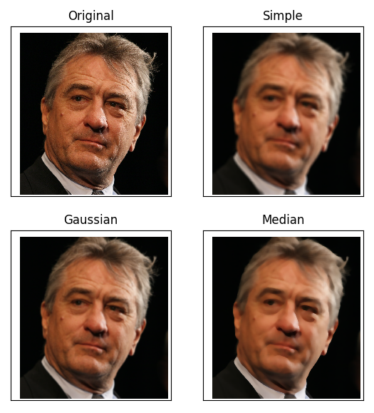
Suppose we have read the input image using the following commands:

import cv2import numpy as npimage = cv2.imread('robert_de_niro.jpg')

The first method, which is the simplest, is simple averaging. In this method, the value of each image pixel is replaced with the average of the values of the pixels inside a window around that pixel.

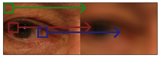
By doing this, the amount of noise in each pixel becomes the approximate average amount of noise, which naturally is close to zero. To do this, the following command is enough:

simple = cv2.blur(image, (21, 21))

Of course, the two numbers 21 in this command are the length and width of the window I introduced.

The next method is using a Gaussian kernel. Did you notice that in the simple method, the values of the pixels inside the window corresponding to each pixel contributed to producing the output with equal weight? Now if these weights are computed based on the distance of each pixel from the central pixel (the one whose value will be replaced by the average) and the Gaussian distribution function, we will have Gaussian blurring. In general, this method gives a more human-pleasing result than simple averaging. This too can be executed with one command:

gaussian = cv2.GaussianBlur(image, (21, 21), 0)

But that zero after the window dimensions! This number tells OpenCV to take the standard deviation of the values inside the window into account for computing the weight.

Another solution is that in that infamous window, instead of computing the average, or weighted average, we compute the median. The median of a series of numbers is the number that falls in the middle of their sorted list. For example, for the numbers 2,3,4,4,4,5,12,16,25 and 255, the median value is 5. This method is useful for removing salt-and-pepper noise (noise in which the noise values are either very large or very small, for example random black and white dots that we sprinkle randomly in the image.) This one too is a single line of command:

median = cv2.medianBlur(image, 21)

In the case of the median, the dimensions of the desired window must definitely be square, which is why only one number represents the size of the window. Of course, this limitation is not theoretical; this is how OpenCV’s implementation is.

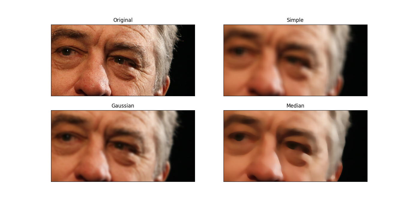
For a better comparison, see a zoomed-in version:

Extracting Image Edges

One of the important pieces of information inside images is the edges present in them. Image edges are usually obtained by computing the gradient (multidimensional derivative). Now, in different methods, different disasters befall this poor gradient so that the edges become visible.

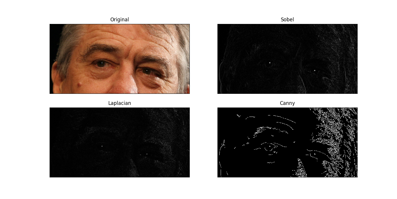
One of the edge detection methods is using the Sobel operator. In this method, the values of a 3 by 3 window around each point are considered, and the (weighted) values of one side of this window are subtracted from the other side. More precisely, depending on the direction of applying the differentiation, a kernel like the following is used for computation:

$$K=\left[\begin{array}{ccc}-1& 0& 1\\ -2& 0& 2\\ -1& 0& 1\end{array}\right]$$

This operation is also of the same kind as blurring; only half of the weights are negative. The command for this one is:

sobel = np.absolute(cv2.Sobel(image, cv2.CV_32F, 1, 0)).mean(2)

Another method is using the Laplacian. To put it more briefly than the Sobel operator, in this method the following kernel is used!

$$K=\left[\begin{array}{ccc}0& 1& 0\\ 1& -4& 1\\ 0& 1& 0\end{array}\right]$$

And its command:

laplacian = np.absolute(cv2.Laplacian(image, cv2.CV_32F)).mean(2)

And the last, but not the least valuable, method is Mr. Canny’s method. This one is not just a weighted average over windows with fixed dimensions. In this method, first Gaussian blurring is applied to the image, then differentiation is performed. After that, the obvious noise is thrown away, and finally two thresholds are applied with hysteresis. In short, it is quite a hassle to obtain edges this way, but well, in return, among the usual methods, this one is almost the best!

canny = cv2.Canny(image, 100, 200)

The two numbers 100 and 200 are the threshold values for hysteresis. When the derivative value in a pass — moving over the pixels of the image — becomes greater than the upper limit — here 200 — that point is considered part of the edges, and as long as the derivative value does not fall below the lower limit — here 100 — the points continue to be considered edge points.

A Cute Example

So far we have seen what averaging — the same blurring — and differentiation do to an image. Now if we want to make the image smoother but not destroy the important edges so that the image remains clear, what should we do?

My proposed method is to first find the edges of the image, then blur them so that we have a matrix whose values are one at the edges, gradually move toward zero around the edges, and are zero in regions farther away from the edges. This way we can preserve the original image in these regions and put the blurred image in the remaining regions.

For this purpose, we start with the Sobel operator:

edges = np.absolute(cv2.Sobel(image, cv2.CV_32F, 1, 0)).mean(2)

Then we place its values between 0 and 1 in such a way that the largest value is mapped to 1 and the smallest to zero:

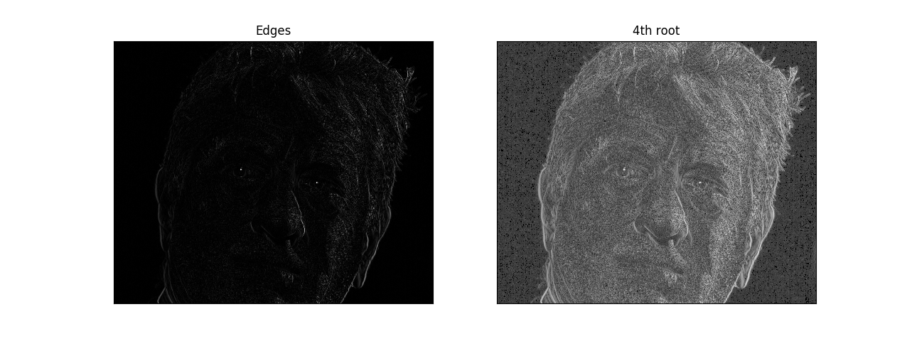
edges = (edges - edges.min()) / (edges.max() - edges.min())

Now, so that more areas of the original image are preserved, we take the fourth root of the obtained values. By doing this, values close to 1 become closer to one, and only places where the numbers are truly close to zero remain near zero:

edges = edges ** 0.25

You can see the effect of this operation in the image below:

Well, now we also need to create a blurred version of the image:

blurred = cv2.medianBlur(image, 21)

Finally, we need to combine the blurred and original images. This is simple given the initial idea. We now have a matrix whose values are between zero and one, and it is closer to one where we have a stronger edge. So it is enough to multiply the values of this matrix by the original image, and 1 minus the values of this matrix by the blurred image, and consider the sum of these two values as the result. By doing this, where our coefficient matrix is close to one, the pixels of the original image are placed, and where it is close to zero, the pixels of the blurred image. In the remaining regions, we will have a combination of the original and blurred images, which is closer to the original image the stronger the edge is in those regions, and otherwise closer to the blurred image.

edges = np.expand_dims(edges, 2)edges = np.tile(edges, (1, 1, 3))blurred = cv2.medianBlur(image, 21)final = (1 - edges) * blurred + edges * imagefinal = final.astype(np.uint8)

In the code snippet above, the first two commands are only there because the tensor of our original and blurred image is 3-dimensional, while the edge coefficients are 2-dimensional. This is because the original and blurred images are color images and have 3 red, green, and blue channels, while the edge coefficients only change with the pixel coordinates on the image and must be the same for all 3 channels. I have done exactly this in the first two commands of the code snippet above. The first command adds a dimension to the coefficients, and the second repeats the coefficients 3 times along this dimension. The last command is only for converting the data type so that OpenCV considers our image a normal 3-channel image.

By carrying out these steps, the job is done. You can see the result in the image below:

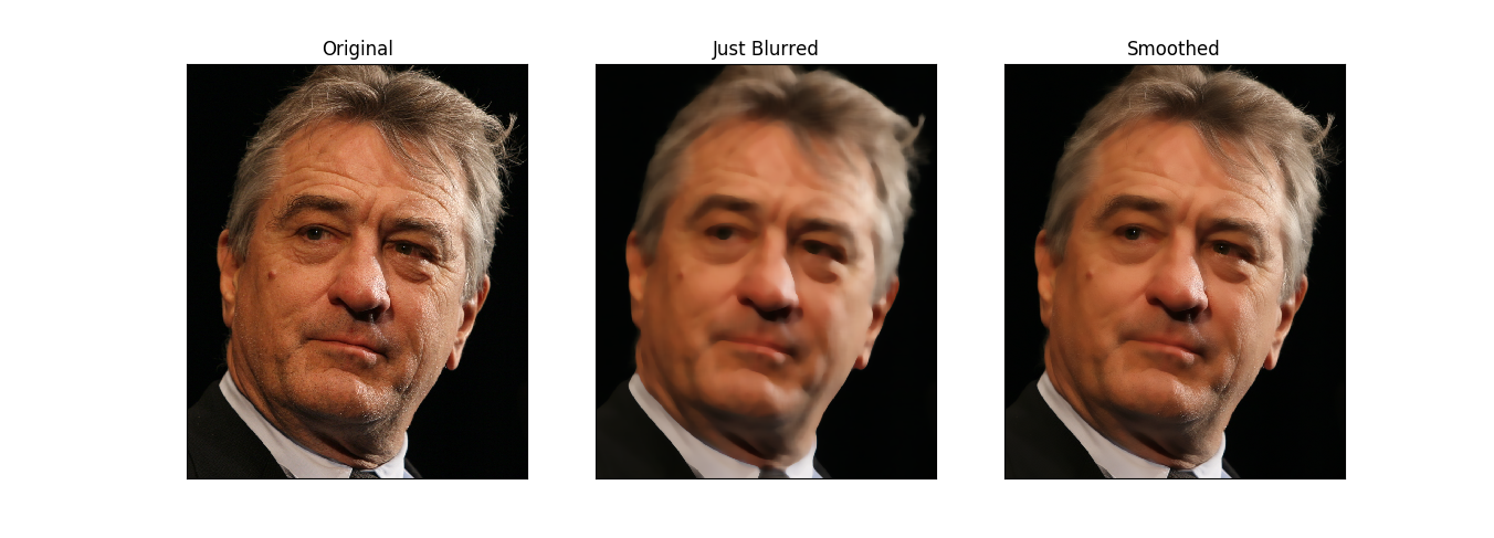
To make a proper comparison possible, I have put the original image on the left, the blurred image in the middle, and the combination of the two, which is the final result, on the right. You see, with a set of suitable operators, a cute result can be obtained!

The codes related to this post are available in two versions, python and c++‎, from here.