Measures and Integrals: Stochastic Processes

Written on November 7, 2017

NOTE: This post is automatically translated from Farsi using GPT 5.5

Stochastic processes are familiar to students in many fields: electrical engineering, artificial intelligence, aerospace engineering, economics, and the like. All functions whose values, from our point of view, are random numbers fall within the set of stochastic processes. The values of an electromagnetic signal that reaches a mobile phone, a company’s stock value over time, the amount of displacement of a component in a mechanical system—all of these are stochastic processes.

Stochastic processes, like integrals, can also be studied within a non-rigorous framework; however, studying them within the framework of measure theory is more solid and brings better perspectives to the learner (good on it!)

Now let’s examine a problem related to these very stochastic processes. Suppose we want to compute the integral of a function $f$ over a particular interval (say, 0 to 1), but we do not have the function itself. What we have are samples of values of $f$ that we have been able to measure. This problem is entirely practical. We usually do not have complete information about the functions we deal with, and only limited measurements of them are available to us.

One initial and useful solution is to connect the points we have with straight lines. In this way, we have a piecewise-linear function whose integral we can compute. Or we can pass a quadratic curve through every three points and approximate this way. Many of these methods are taught to students in undergraduate numerical analysis courses.

But what if we have information about the function $f$ that is probabilistic? Can we use it in reconstructing the function or integrating the function? What does probabilistic information about functions even mean?

This is where measures show up. With common tools, it is not easy to measure a set of functions (for example, assign probabilities to them.)

Warning The problem raised above (integrating an unknown function) is not on the agenda here. From here on, the discussion concerns measures on sets of functions, and in particular we examine Wiener measure, which is the probability law of the Wiener process.

Wiener Measure

Mr. Wiener, whom you are surely familiar with. The Wiener filter is named in his honor. Mr. Wiener was an American mathematician and philosopher who was a professor at MIT. He was among the first people who tried to examine the properties of sample functions of stochastic processes as well. If it is not clear from the name, the sample functions of a stochastic process are the functions we encounter if we know exactly the state of the events that have caused a process to become random — if we sit in God’s place! —. For example, if I know the state of a communication channel — such as an urban environment — exactly, the electromagnetic signal received by the mobile phone becomes a simple function of time for me. Between us, there is no need to sit in God’s place; our very mobile phones are practically dealing with sample functions. The signal that reaches the mobile phone is not known to us beforehand; but when it reaches the mobile phone, it has definite values, so it is a sample function.

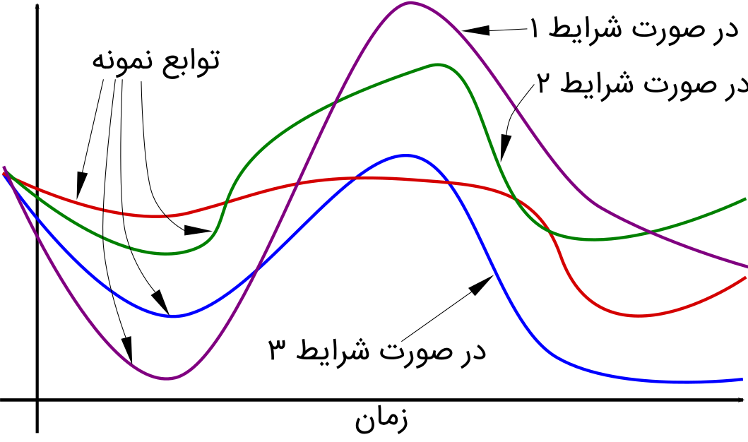
Finding the properties of the sample functions of a stochastic process is a very attractive problem. Mr. Wiener proposed a Gaussian measure for the probability of occurrence of sets of these functions.

If we have come this far together correctly, you should ask: well, on what sigma-field is this measure defined? Suppose we know that the functions we have in mind have values in particular intervals at times $t_{0}$ , $t_{1}$ , and so on up to $t_{n}$ . For example, at time $t_{0}$ the value of the functions of interest to us lies in the interval $(5,10)$ , at time $t_{1}$ in the interval $(8,11)$ , and so on. For these intervals, too, we take the names $A_{0}$ through $A_{n}$ . With these facts in hand, we have effectively described a subset of the sample functions of the stochastic process: among all sample functions, those that, at specified times, take values in specified intervals. For ease of work, let’s give this subset a name:

C (t_{0}, \dots, t_{n}; A_{0}, \dots, A_{n})

Now we define the value of the measure for these subsets:

\begin{matrix} μ (C (t_{0}, \dots, t_{n}; A_{0}, \dots, A_{n})) = \\ \int_{A_{0}} \int_{A_{1}} \dots \int_{A_{n}} p (t_{n} - t_{n - 1}, x_{n} - x_{n - 1}) \dots p (t_{0}, x_{0}) d x_{n} d x_{n - 1} \dots d x_{0} \end{matrix}

The function $p$ is also the same Gaussian form, namely $p (a, b) = (4 π a)^{- n / 2} e^{- | b |^{2} / 4 t}$ .

With this measure in hand, we can do interesting things. For example, what function is the expected value of the square of functions that have the Wiener probability distribution? Note that we have not specified any particular subset, so we have neither values of $t_{i}$ nor a bounded interval $A_{i}$ :

𝔼 (| ω (t) |^{2}) = \int p (t, x) | x |^{2} d x = 2 n t

So the expected value of the magnitude of the sample function of a process with this law becomes $\sqrt{2 n t}$ .

A process whose probability law is the Wiener measure is called a Wiener process (isn’t that obvious?)

The Wiener process has widespread applications in financial mathematics and physics.

Final Word

It seems that, without intending to, I have developed a special fondness for trilogies. In any case, in my opinion, continuous discussion of measures beyond this is not suited to the patience of personal blog posts like mine. The purpose of this series of posts was to increase the curiosity and interest of a possible reader in the foundational topics of modern probability theory, to present a practical example of the benefits of changing one’s viewpoint in this style, and finally to examine a problem more advanced than ordinary probability, which itself is also in line with motivating further study in this area and is practically part of the first goal.

Apology In the first version of the first post in this series, the images I had included were wrong. In fact, they incorrectly depicted the operation of integration, which had been explained correctly. These images were corrected as soon as the second post was published.