Measures and Integrals: Eyes Must be Washed

Written on October 5, 2017

NOTE: This post is automatically translated from Farsi using GPT 5.5

If you are, or have been, a graduate student in engineering or mathematics, you have surely come across integrals of the form

$${\int }_{D}f(x)d\mu (x)$$

Especially if you have reached statistics and probability in serious and recent papers, which is also quite likely.

The first time I encountered this kind of integral was during my master’s program at the Electrical Engineering department of Amirkabir University. From the very first year, when I was reading papers by people like the great Thomas Kailath or Simon Haykin, these integrals seemed strange to me, and lovable. Well, to be honest, my excessive interest in mathematics is surely evident from my appearance and writings; but even if that interest had not been there, seeing these integrals would still have aroused my curiosity. In artificial intelligence too, Professor Vapnik’s readable book “Statistical Learning Theory” has many integrals of this sort.

Apparently, the new way of dealing with integrals was initiated in the final years of the nineteenth century by Émile Borel — the great French mathematician. A theory that was later developed by Henri Lebesgue — another great French mathematician — and shook the foundations of mathematical analysis.

Setting aside this brief bit of historiography, the first thing I want to say in this regard is why, when we know Riemann integrals and their predecessors and have learned them in high school and the first year of university, should we involve ourselves in understanding another kind of integral?

The first answer to the question above is: there is no need! For someone who is living well with what they know today and seeks excitement in life through discovery and exploration in other domains and fields, doing this is a waste of resources. But if — as I mentioned above — you deal with these integrals in your work or interests, the answer is that the new type of integrals have greatly improved mathematical analysis. They have transformed probability theory. And finally, through creating greater abstraction, they have made it possible to study new subjects.

It is clear that somewhere like my daily writings, there is neither the opportunity nor the possibility to examine this theory precisely. My intention is that in this post and the posts following it, I open up the subject to some extent from a general perspective and create more curiosity.

One Must Wash One’s Eyes

We remember from high school that when we wanted to calculate the area under a curve specified by $f(x)$, we would divide its domain into very small pieces and, in each piece, calculate the value of $f(x)$ at an arbitrary point and approximate the area of that small piece under the curve with the area of the small rectangle that was formed

and by making the width of the rectangle smaller, we would improve our approximation. The limit of these approximations, when the number of rectangles is infinite, was the area under the curve:

$$\int f(x)dx={\text{lim}}_{n\to \infty }\sum f(x_i)(x_{i+1}-x_i)$$

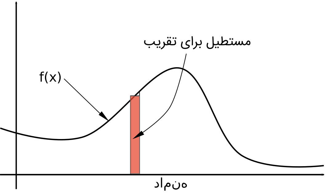
But this procedure has several problems. One is that the validity of this approximation is only for when the domain over which the integral is calculated is bounded. In practice, to calculate integrals over unbounded domains, we are forced once again to calculate the limit of the calculation of the bounded integral. Second, when this unbounded domain is combined with another unbounded domain — for example, when we calculate a double integral $\int \int$ — all sorts of technical problems arise for the calculation.

Now let us look at it differently. If instead of dividing the domain, we divide the range of the function, and then for each piece of the function’s range, consider the area of all the rectangles that are formed, what happens?

Again, intuitively, we can calculate the area under the graph by summing the areas of these rectangles. The trick that makes this method of calculating the integral so different is that instead of considering these rectangles separately, we consider a “measure” that measures those parts of the function’s domain where the values of the function fall within our desired range

In the example of Figure 3, we can calculate the area of all the rectangles with the following expression:

$$\text{area}=y_i\mu (A)$$

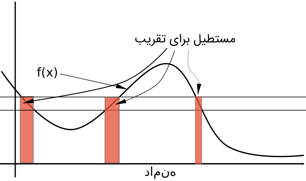
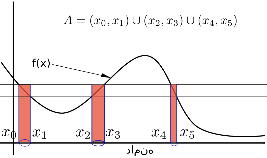
where $A$ is the same subset of the function’s domain that has been separated by the blue ellipses, $\mu$ is the measure function that measures the size of this subset, and $y_i$ is the value of the function on this subset of the domain.

This simple trick makes it possible to perform many operations. Again in the example of Figure 3, if the function $\mu$ returns the value $|x_1-x_0|+|x_3-x_2|+|x_5-x_4|$ for $A$, the value of the integral we calculate will be exactly equal to its Riemannian version. But this is not the only useful measure for integrating the function $f$. Another important example of useful measures is the probability distribution measure.

Let us suppose that the probability that the input of our function — the same $f$ — lies in certain intervals is known. Also suppose that we name this measure $P$. In mathematical language, what we have said becomes:

$$P(x\in A)=\mu (A)$$

Now we can calculate another integral. The value of this integral is the expected value of the function $f$. Previously, to calculate the expected value of the function $f$, we first obtained the probability density function, which was equal to $p(x)=\frac{dP}{dx}$; then we calculated the following integral:

$$𝔼(f(x))=\int f(x)p(x)dx$$

But with the new form, we can write:

$$𝔼(f(x))=\int f(x)dP$$

In this form, $P$ does not even need to be differentiable. The domain of our function does not need to be one of the well-behaved kinds of domains we had dealt with before. For example, the domain of our function can itself be a set of functions. Functions whose domain is itself a set of functions are known in mathematics as functionals.

You see! With a change in perspective, a new field for research and application was found. The study of functionals. If you think these are a bunch of impractical abstractions that mathematicians amuse themselves with, I refer you to the same names I mentioned at the beginning of this post. Vapnik and Kailath and Haykin. All of them, in addition to being good mathematicians, have done most of their work in applied areas. The last two were, and are, practically electrical engineers and have worked in the field of signal identification. The very thing that has made it possible for us now to take our mobile phones out of our pockets wherever we want and call someone we love.

In fact, if even these cannot properly reveal the applicability of this area of mathematics, I will give an example of these functionals. The familiar Fourier transform function is a functional. You remember that this functional took a continuous function and a real value and returned another real value:

$$F(f,\omega )=\int f(x)e^{j\omega x}d\mu (x)$$

What is meant by $\mu$ in the formula above is the Lebesgue measure. The same one that, for the set $A$ in the example of Figure 3, returns the value $|x_1-x_0|+|x_3-x_2|+|x_5-x_4|$.

I hope that up to this point I have been able to create the necessary curiosity to continue talking about measure theory and integration. In the following posts, we will look a little — only a little — more deeply at measure theory and also examine one or two practical examples; may it be useful to someone!