Trainable Models: Line, The Simple Righteous Function

Written on August 5, 2017

NOTE: This post is automatically translated from Farsi using GPT 5.5

In the previous part, I wrote about the computer and how it learns. In the middle of that write-up, I mentioned my simple and dear friend, the straight line. That despite its limited abilities, it can be useful and make the computer learn things.

I think now is the time to spend a little time seeing the real result of a simple training using this righteous function.

Imagine people from two tribes have built homes for themselves in a geographic region. After a while, a disagreement has arisen over which part of that region is each tribe’s territory. And who knows how our computer has ended up in that time, where tribes like this existed and got into conflicts with each other.

Now we want to show our computer the points where the people of these two tribes have built houses, and from then on the computer will tell us which tribe each point in that region belongs to. (For God’s sake, don’t nitpick my problem statement; ridiculous as it is, I thought a lot before I came up with it!)

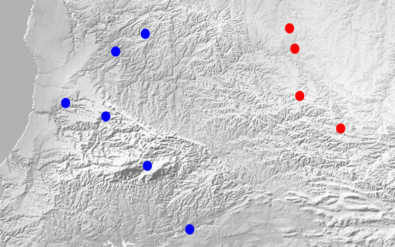
So we have a number of points representing the locations of the blue tribe’s houses and a number of points representing the red tribe’s houses. The straight line, which we saw in the previous post, has two parameters. One represents the slope of the line and the other its y-intercept ( $a$ and $b$ in the formula $y = f (x) = a x + b$ .)

In the classroom, the appropriate values of $a$ and $b$ should be learned such that it has the greatest distance from the houses of the red and blue tribes, and at the same time each tribe lies on one side of the line corresponding to these parameters.

With one look at the formula of a straight line ( $y - a x - b = 0$ ), we can guess the result of several points being on one side of the straight line. If we put the coordinates of points that are on the straight line into the formula, that is clear and the number zero is obtained. But if several points are on one side of the line, the sign of the value obtained by putting their coordinates into the formula will be the same.

So let’s agree that the sign of the red tribe is negative and the sign of the blue tribe is positive. Apparently things are moving along. Only one point remains. The straight lines that can separate two sets of points are countless.

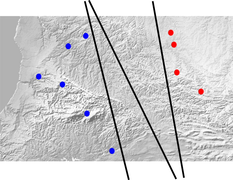
Each of the black lines in the image above could be an answer. Of course, one point had been forgotten! This line was supposed to have the greatest distance from the houses of both tribes. For this last condition to be met, instead of one separating line, we consider two separating lines. One of them has gone as far as the nearest possible point of the blue tribe and the other as far as the nearest point of the red tribe, and both are parallel. These two lines represent the distance of the single boundary line from each of the tribes. Now it is enough for the distance between these two lines to be maximized. The final separating line will be the average of these two lines.

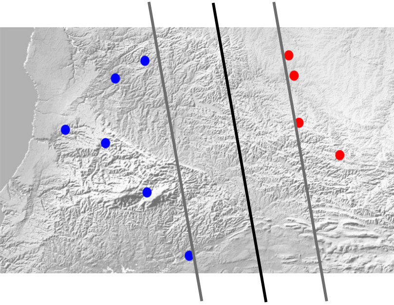
Since we said the support lines are parallel, their parameter $a$ is the same. But they do not have the same y-intercept. For example, the y-intercept of one of them is $b_{0}$ and the other is $b_{1}$ .

Our problem can be expressed as follows:

\begin{matrix} Maximize \frac{| b_{0} - b_{1} |}{1 + a^{2}} \\ subject to & l_{i} (y_{i} - a x_{i} - 0.5 (b_{0} + b_{1})) > 0 \end{matrix}

The meaning of the relation above is: maximize the value $\frac{| b_{0} - b_{1} |}{1 + a^{2}}$ while, for all points (whether belonging to the red tribe or the blue one), the value of that point’s sign (the sign corresponding to the tribe — $l_{i}$ ) multiplied by the value obtained by putting the point’s coordinates into the line formula is positive. This means the line correctly predicts the tribe label.

Ouch! Yet another problem! And that too for a simple problem like this. What has been obtained so far is not a convex problem, and optimization toolboxes cannot solve this problem with a proper guarantee. But the solution to the problem is not difficult. It is enough to write our straight-line formula in another way. We have seen this in high school too:

a y + b x + c = 0

By doing this, an unnecessary degree of freedom is added to the line formula. But this same unnecessary degree of freedom can solve many problems. To represent the support lines, we do not need to keep their y-intercepts in mind. This time we take the main separating line to be $a y + b x + c = 0$ and the two support lines as:

\begin{matrix} a y + b x + c - 1 = 0 \Leftarrow y - (- \frac{b}{a}) x - (- \frac{c - 1}{a}) = 0 \\ a y + b x + c + 1 = 0 \Leftarrow y - (- \frac{b}{a}) x - (- \frac{c + 1}{a}) = 0 \end{matrix}

Note that although a degree of freedom has been added to the straight-line formula, the total degrees of freedom of the problem have not changed!

Now our problem becomes:

\begin{matrix} Maximize \frac{| 2 |}{a^{2} + b^{2}} \\ subject to & l_{i} (a y_{i} + b x_{i} + c) > 0 \end{matrix}

By taking one more step, we arrive at a convex problem; it is enough for the form of the objective function to be inverted:

\begin{matrix} Minimize a^{2} + b^{2} \\ subject to & l_{i} (a y_{i} + b x_{i} + c) > 0 \end{matrix}

The existing optimization tools solve this problem easily, and once the riddle is solved, it seems simple. Now whenever a problem arises between the tribes, it is enough to give the point of dispute to the computer so that it obtains its sign and says which tribe it belongs to.

So that those interested in following these topics can see in practice how to grapple with this problem, I have written a sample program in Python which, if you give it the image of the map and the tribes, will find the boundary line for you.

If you get the program and run it, you will see the following result

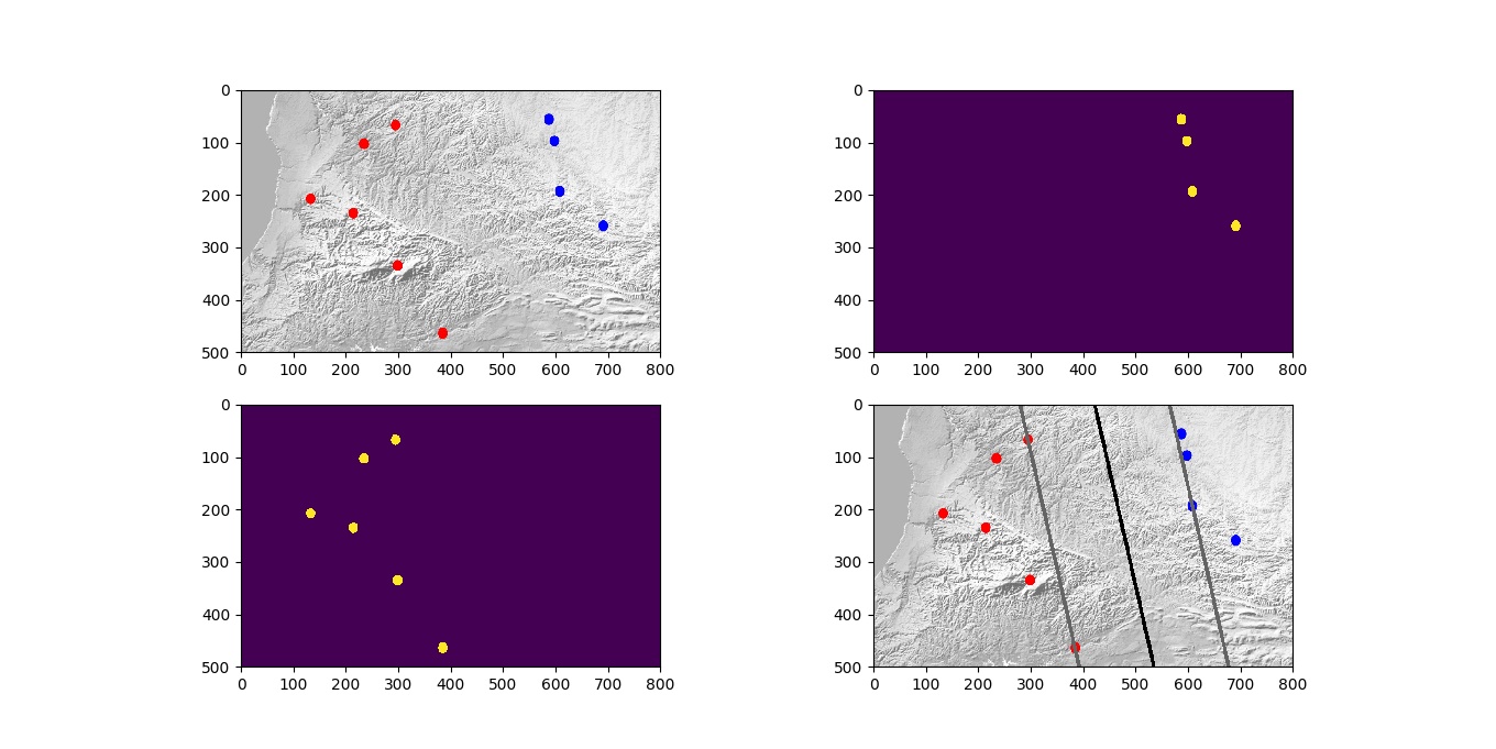
To run the program, you need to install a few libraries. The first library is the OpenCV library for Python. Assuming you live on the Ubuntu — or Mint — operating system, the following command installs this library

sudo apt-get install python-opencv

The next libraries are matplotlib, numpy, cvxopt, and cvxpy. You can install all of these with the following commands

sudo supip install --upgrade pippip install --upgrade matplotlibpip install --upgrade numpypip install --upgrade cvxoptpip install --upgrade cvxpy

Now it is enough to clone the program from git or download it from the GitLab address, and then run it with the following command

python doit.py

Inside the program’s code, I have also put a brief explanation for each section, which I hope will be useful.