Trainable Models: This Clever Computer—How on Earth Does It Learn?

Written on November 13, 2016

It was the year 1373 in the Persian calendar when I acquired my very first personal computer. To be more precise, it was purchased for me. Back then, the RAM in those devices hovered around a mere 1 megabyte, and the most “intelligent” feat this lovable invention could muster for me was capturing keystrokes and catapulting Aladdin right over the Caliph’s guards in a game.

Oh, how computers have evolved since those days! They’ve shrunk in size, much like us humans—compact and ever more capable. Nowadays, you can chat away with your mobile phone, making requests as if it’s an old friend. Or, in some foreign land, you might snap a photo of a road sign, show it to your device, and politely ask it to read the thing aloud—in your own tongue, no less.

But how on earth is that possible? A bunch of clueless flip-flops and a few dozen grams of semiconductors figuring out how to see and hear? It’s enough to make you wonder if these machines have been sneaking peeks at philosophy books.

Mathematical Functions from a Fresh Perspective

The very first type of mathematical function we’re typically introduced to—at least, if memory serves—is the straight line. The function $y = m x + b$ , if I’m not mistaken. At any rate, it’s the inaugural operational function we encounter: one with a single variable, sketching a smooth line across a two-dimensional plane, like a sheet of paper. Depending on the values of $m$ and $b$ , the line’s position and slope shift accordingly.

A lone straight line might not accomplish grand feats on its own, but even with its modest toolkit, it can achieve remarkable things—especially when we enlist a substantial number of them. For instance, with just one line, you can neatly bisect a two-dimensional plane into two utterly distinct halves: one side for the “baddies,” the other for the “goodies”! And if you’ve got enough lines at your disposal, you can carve up that plane however your heart desires.

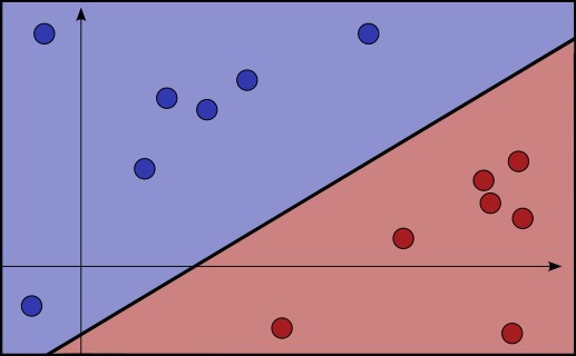
Computers, too, often view functions through this very lens—particularly when it’s time for learning. We start with a general function boasting a plethora of parameters. As we train it, the system learns optimal values for those parameters, fine-tuning them to deliver results that align more closely with our expectations. Naturally, what we aim to sort into “good” and “bad”—or a multitude of other labels—isn’t some simple two-dimensional sheet. Yet the underlying mechanism mirrors that plane-splitting trick precisely.

Researchers have crafted and tested a dazzling array of these general functions over the years. Think Artificial Neural Networks, Support Vector Machines, fuzzy functions, Probabilistic Graphical Models, and the like. I must emphasize again: from the machine-learning vantage, they’re all functions laden with parameters galore. These are models that operate on hyper-dimensional spaces—spanning tens or hundreds of thousands of dimensions—with parameter counts soaring even higher.

So, How Do We Train Our Function?

To unpack this properly, let’s circle back to our trusty straight-line example: $y = m x + b$ . This time, I’ll split the function’s inputs into two camps: the core inputs (our $x$ ) and the parameters ( $m$ and $b$ ). Mathematically and computationally speaking, these two input types are indistinguishable. In practice, they’re equals too. The distinction is merely a design convenience, ensuring we feed the right values to the right spots. If you’re a programmer, you’ve doubtless tangled with naming conventions—clever use of this principle can elegantly resolve the puzzle of function training.

Before we dive headlong into the training pool, a quick aside: teaching a computer bears uncanny resemblance to tutoring a human pupil. Here, too, we need a teacher and a hearty helping of training data for the machine to observe and absorb, learning what to do. Say, for instance, we prepare a dataset of images where we’ve meticulously marked spots containing text. We feed these to the computer, and voilà—it picks up how to spot text locations in fresh images. Perhaps next, it deciphers the words and reads them back in our language.

Let’s assume our training set comprises samples in the form $(x_{i}, y_{i})$ . For training, we craft a fresh function that takes only $x_{i}$ and $θ$ (our parameters) as inputs. We’ll christen it the error function and denote it as $L (θ; x_{i}, y_{i})$ .

Now, with the guidance of our esteemed teacher, we hunt for the $θ$ that minimizes $L$ . In other words, values that best fulfill our desired outcomes. If you scrutinize the formula, it computes the gap between the function’s learned output and our target $y_{i}$ , squares it for good measure (to keep things positive), and sums these discrepancies across all samples we’ve shown the machine. A tiny total means each term in that sigma summation was puny—since they’re all non-negative.

And who, pray tell, is this erudite teacher? None other than the “optimization toolkit.” A treasure chest assembled by optimization scholars in mathematics and engineering. If this piques your curiosity, I warmly recommend Stephen Boyd’s book—one of the field’s most affable luminaries. But as a practitioner, you needn’t delve too deep: the algorithms exist, the toolkits are coded, and for straightforward problems like linear programming (as Boyd himself quips), they’ve evolved into indispensable technology. In broader cases, you can wield them effectively without becoming an expert.

The tale’s grown long, and patience has its limits. May your days brim with vitality and wonder.